If we knew what we were doing, it wouldn’t be called research.
- Albert Einstein
This post marks the beginning of a series where I document my undergraduate research — the experiments, the failures, and what I learned. If you’re here from the future (after I’ve posted the follow-ups), you’ll find links below. If not, bookmark this and check back.
The series is broken into the following parts:
- Hitting My First Roadblock: Where Did the Gradients Go?
- Healthy Gradients, Unhealthy Confidence
- What I’d Do Differently (And What the Data Was Telling Me All Along)
A little about the FEM domain
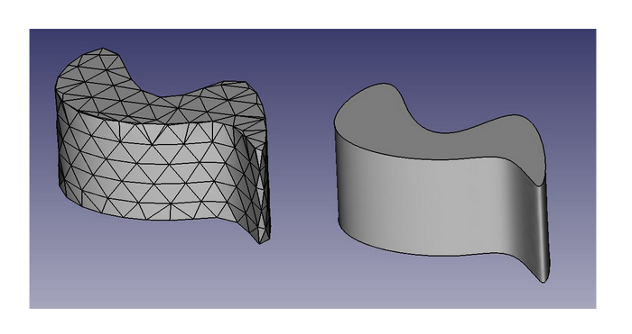
FEM, or the Finite Element Method, is the backbone of structural simulation. The core idea is deceptively simple: take a complex structure, break it into thousands of tiny elements (a mesh), solve the physics on each one, and assemble the results to understand how the whole thing behaves under load.
It’s used everywhere — from crash testing car bodies to analyzing stress in aircraft wings. If something needs to not break under pressure, there’s a good chance someone ran an FEM simulation on it first.
The Pain Points of FEM
Powerful as it is, FEM has a cost — and it’s not a small one.
It’s slow. Running a single simulation on a complex mesh can take hours, sometimes days, depending on the fidelity you need. If you’re doing design optimization — iterating over hundreds of configurations — that cost compounds fast.
The mesh matters. A poorly generated mesh doesn’t just give bad results, it can make the solver fail entirely. Getting it right often requires domain expertise and manual intervention.
Boundary conditions are finicky. How you constrain a model (where it’s fixed, where force is applied) directly determines what you get out. Small mistakes here cascade into large errors downstream.
My research was specifically aimed at the first problem: the computational cost. The question I was trying to answer — can a machine learning model learn to approximate what FEM computes, without actually running the solver?
The Problem Statement
The goal was to train a surrogate model that could predict nodal displacements on a structural mesh given the loading and boundary conditions — effectively learning the input-output mapping of a static FEM run.
If it worked, you’d get simulation-quality predictions in milliseconds instead of hours.
MeshGraphNets: A seemingly promising direction
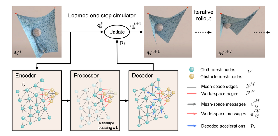
The architecture I chose was MeshGraphNets (MGN), introduced by DeepMind in this paper. The core idea is elegant: represent the mesh as a graph — nodes are mesh points, edges encode connectivity — and train a GNN to propagate information across that graph the same way physics propagates through a structure.
This is called message passing. Each node aggregates information from its neighbors, updates its own state, and the process repeats for several steps. Over enough iterations, local interactions compound into global understanding of how the mesh deforms.
It felt like a natural fit — the graph structure of a GNN mirrors the mesh structure of FEM almost directly.
Why MeshGraphNets?
There were a few GNN-based surrogate approaches I looked at, but MGN stood out for one reason: it was designed specifically for mesh-based simulations. Most GNN architectures treat graphs abstractly — MGN treats the mesh as a physical domain, encoding edge features like relative position and distance that matter for structural problems.
It also had DeepMind’s empirical backing across fluid and structural domains, which gave me reasonable confidence it wasn’t a shot in the dark.
The Data Problem
This is where things get genuinely hard — and it’s something that doesn’t get talked about enough in ML research that touches simulation.
Creating a single simulation-ready mesh isn’t just drawing a shape and hitting run. You need to make decisions about element type, mesh flow, part behavior, shell thickness (PID thickness in ANSA), boundary condition placement, and load application — and most of these require manual intervention from someone who knows what they’re doing. A bad mesh doesn’t just produce wrong results; it often won’t solve at all.
Now multiply that by the thousands of data points a model needs to train on. Each one is a potential hours-long preprocessing job. For a single researcher with access to a finite set of base geometries, creating a meaningfully diverse dataset from scratch is close to infeasible.
So I went with data augmentation.
I wrote Python scripts using the ANSA Python API to programmatically generate variations from 25 base meshes — ending up with 1000+ data points. The variations were across three axes:
- Morphing: geometrically deforming the mesh to produce shape variations while preserving connectivity — think of it as stretching or reshaping the base geometry parametrically
- Number of holes: structural meshes in sheet metal often have cutouts; varying their count changes the stress distribution patterns the model needs to learn
- Sheet thickness: a direct material property that affects stiffness and displacement magnitude across the whole mesh
The limitation — and I’ll come back to this in the retrospective post — is that augmentation from a narrow base has a ceiling. You can vary parameters all you want, but if your 25 base meshes share the same fundamental topology, your augmented dataset will too. That ceiling matters more than it seems upfront.
Running the Simulations
For the actual FEM solves, I used HPC (high-performance computing) nodes to run the simulations in parallel across the dataset — the only practical way to generate 1000+ results without waiting weeks. Each solved mesh produced three nodal displacement fields that became the model’s training target.