Tensors: The Bricks of PyTorch

First principles, Clarissa. Once you understand the ingredients, you can cook anything. - Massimo Bottura

Tensors illustration. Created with Nano Banana.

I’ve been exploring torch more deeply lately, and if you want to understand what is really happening under the hood, brushing up on tensors is a must.

If you’ve used torch before, tensors probably felt like multi-dimensional arrays that hold data. That description is not wrong, but it is only the surface. Underneath, the story is more careful than that, and once you see it clearly, a lot of PyTorch behavior starts making much more sense.

This is exactly the kind of thing that can feel slippery at first. You slice something, transpose something, reshape something, and suddenly you are left wondering why the values are behaving differently from what you expected. Usually the confusion is not in the data itself. It is in how the tensor is looking at that data.

What’s a Tensor?

Think of a tensor as an object, a reference that carries properties describing how it relates to the actual data it represents. It is not the data itself. It is metadata layered on top of a flat memory buffer.

A tensor has six core components:

tensor
├── storage   # the actual flat memory
├── dtype     # what type of data lives there
├── shape     # how elements are arranged
├── stride    # how to navigate dimensions
├── offset    # where the view begins
└── view      # the logical lens over storage

Let’s go through each one.

Storage

Storage is the raw, flat memory buffer that holds the tensor’s elements. This is the first big idea worth holding onto:

Two tensors can point to the same storage.

This is possible because a tensor does not own its data. It holds a reference to a memory location. That is what makes operations like slicing and transposing so cheap: no data needs to be copied, just a new tensor object with different metadata gets created.

Try this in PyTorch:

import torch

base = torch.arange(12)
view = base.view(3, 4)
slice_view = view[:, 1:]

print("base:", base)
print("view:\n", view)
print("slice_view:\n", slice_view)
print("same storage (base/view):", base.untyped_storage().data_ptr() == view.untyped_storage().data_ptr())
print("same storage (base/slice_view):", base.untyped_storage().data_ptr() == slice_view.untyped_storage().data_ptr())

base[1] = 999
print("\nafter mutating base:")
print(view)
print(slice_view)

Dtype

This is the type of the elements: int8, float32, bfloat16, and so on. It deserves its own post, but for now the main thing to remember is that dtype decides how many bytes each element occupies and how those bytes should be interpreted.

Try this in PyTorch:

import torch

x = torch.tensor([1, 2, 3], dtype=torch.int8)
y = torch.tensor([1.0, 2.0, 3.0], dtype=torch.float32)
z = torch.tensor([1.0, 2.0, 3.0], dtype=torch.bfloat16)

print(x.dtype, x.element_size(), "byte(s) per element")
print(y.dtype, y.element_size(), "byte(s) per element")
print(z.dtype, z.element_size(), "byte(s) per element")

View

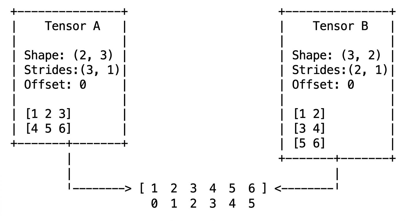
A view is a logical lens over the storage. It does not hold any data by itself. Instead, it carries metadata: shape, stride, and offset. When multiple tensors point to the same storage, what differs between them is the view.

Try this in PyTorch:

import torch

x = torch.arange(6)
a = x.view(2, 3)
b = a.t()

print("a:\n", a)
print("b:\n", b)
print("same storage:", a.untyped_storage().data_ptr() == b.untyped_storage().data_ptr())
print("a stride:", a.stride())
print("b stride:", b.stride())

Shape

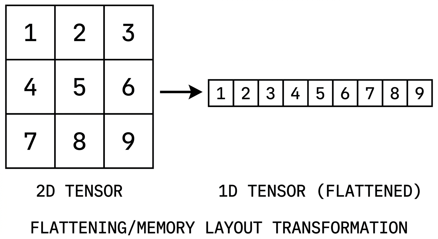
Shape is the tuple that tells you how elements are arranged for a given view.

Given a base storage of 12 elements:

base: [0  1  2  3  4  5  6  7  8  9  10  11]

The same 12 elements can be viewed in multiple ways:

View 1: shape(3, 4)       -> 3 rows, 4 columns
View 2: shape(2, 3, 2)    -> 2 blocks of 3x2
View 3: shape(2, 2, 3)    -> 2 blocks of 2x3

The data does not move. Only the interpretation changes.

Try this in PyTorch:

import torch

base = torch.arange(12)

print(base.view(3, 4))
print()
print(base.view(2, 3, 2))
print()
print(base.view(2, 2, 3))

Stride

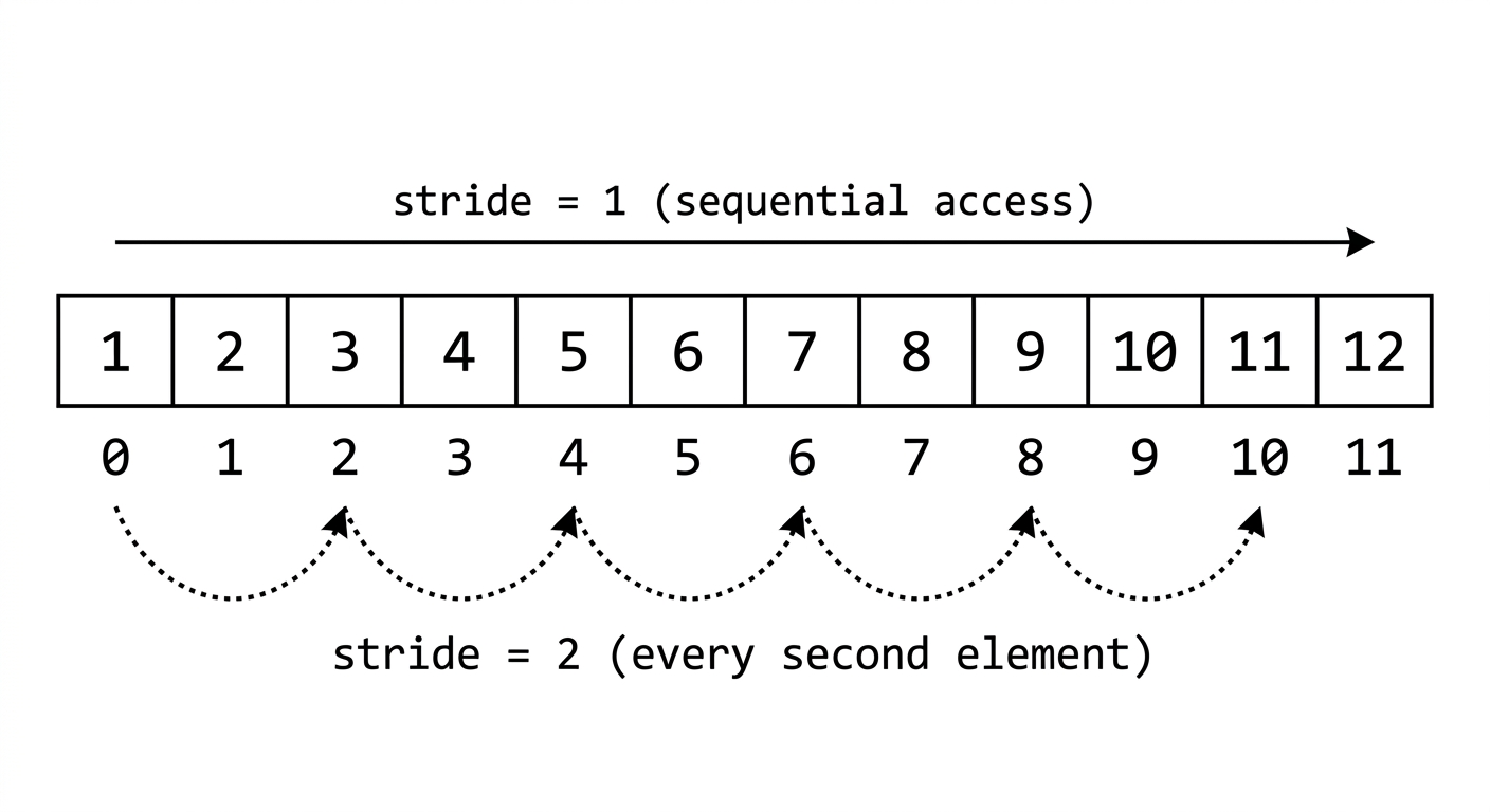
This is where tensors start becoming genuinely fun.

Stride tells you how many elements to jump in flat memory when you move one step along a given dimension.

For a tensor with shape $(d_0, d_1, \ldots, d_n)$ , the stride formula is:

$\text{stride}[d_n] = 1$

$\text{stride}[d_i] = \prod_{j=i+1}^{n} d_j$

Take this example:

base: [0  1  2  3  4  5  6  7  8  9  10  11]

shape(2, 3, 2):

[
  [              <- block 0
    [0,  1],     <- row 0
    [2,  3],     <- row 1
    [4,  5]      <- row 2
  ],
  [              <- block 1
    [6,  7],
    [8,  9],
    [10, 11]
  ]
]

Stride: $(6, 2, 1)$

Jump 6 elements to move from block 0 to block 1
Jump 2 elements to move from one row to the next
Jump 1 element to move along a column (adjacent in memory)

This is row-major layout. Elements within a row are contiguous in memory, which is why the last dimension stride is always 1.

Stride diagram. Created with Nano Banana.

Try this in PyTorch:

import torch

x = torch.arange(12).view(2, 3, 2)
print("x shape:", x.shape)
print("x stride:", x.stride())

y = x.transpose(0, 1)
print("\ny shape:", y.shape)
print("y stride:", y.stride())
print(y)

Offset

Every view has an offset: the index in flat storage where the view begins.

By default, the offset is 0, which means the view starts at the very first element. But the moment you slice a tensor, the resulting view may begin at index 3 or 5 or anywhere else in that same storage.

Here is the formula that maps any multi-dimensional index to its flat storage index:

$\text{storage\_index} = \text{offset} + \sum_{i=0}^{n} \left( \text{indices}[i] \times \text{stride}[i] \right)$

This one formula is what makes the whole system click. Shape, stride, and offset together fully describe any view over any flat memory layout.

Try this in PyTorch:

import torch

x = torch.arange(10)
y = x[3:]

print("x:", x)
print("y:", y)
print("y storage_offset():", y.storage_offset())
print("y stride():", y.stride())

Putting It Together

tensor[i][j][k]
       |
       v
storage_index = offset + i*stride[0] + j*stride[1] + k*stride[2]

A tensor is not just a multidimensional array. It is a structured pointer into flat memory, along with the rules that explain how to navigate it. Slicing, transposing, and broadcasting all follow from arithmetic on these six properties.

Try this in PyTorch:

import torch

flat = torch.arange(12)
x = flat.view(2, 3, 2)

index = (1, 2, 0)
offset = x.storage_offset()
stride = x.stride()

storage_index = offset + index[0] * stride[0] + index[1] * stride[1] + index[2] * stride[2]

print("x[1, 2, 0] =", x[index].item())
print("flat[storage_index] =", flat[storage_index].item())
print("computed storage_index =", storage_index)